Basic Introduction to Matrix Product States
In this tutorial we will give a basic introduction to Matrix Product States (MPS), and show how to efficiently compute tensor-components of an MPS, and overlaps between two MPS.
We’ll be using the following libraries:
import tensornetwork as tn
import numpy as np
import matplotlib.pyplot as plt
The cost of high-dimensional tensors
We begin by analyzing the scaling of the memory cost of storing and accessing elements of tensors with increasing rank and dimension. While the computational complexity of accessing an item in a multidimensional array is \(O(1)\), the main cost is the exponentially growing memory required to store the tensor.
Let our tensor be \(T^{s_1 \cdots s_{\textsf{N}}}\) , where each \(s_i \in \{1, \ldots d_i\}\) and where \(d_i\) is called a physical dimension and \(N\) is rank of the tensor. In condensed matter or quantum computing applications, \(N\) is usually the system size or number the number of qubits. The standard graphical representation of this tensor looks like this,
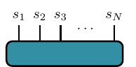
where each line represents one index of the tensor.
Now let’s create a tensor with random entries, with ranks and physical dimensions that run over small ranges, and analyze their memory requirements:
def create_tensor(dimension, rank):
  '''Constructs a tensor of a given rank with random integers'''
  dim_list = tuple([dimension for _ in range(rank)])
  return np.random.random_sample(dim_list)

ranks = range(2,6)
dimensions = range(2,40)

for rank in ranks:
  memory = []
  for dim in dimensions:
      tensor = create_tensor(dim, rank)
      component = tuple(np.random.randint(0, dim, rank))
      memory.append(np.sum([x.nbytes for x in tensor]))
      data = tensor[component]
  plt.loglog(dimensions, memory,'o',ls=':', label = f'N = {rank}')

plt.legend()
plt.xlabel('Dimension')
plt.ylabel('Memory cost')
plt.show()
This produces the following output:
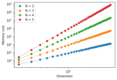
We see that the memory required to store a tensor scales as \(\sim d^{\textsf{N}}\). This is an exponential growth, which quickly saturates our computational resources.
Introducing Matrix Product States
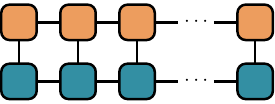
One way to work around this “dimensionality catastrophe” is to focus on a particular kind of tensors: those that can be written as a matrix product state (the word state here is related to the quantum state formed from the coefficients of the tensor). Matrix product states are a special class of tensors that can be written as products over many rank-3 tensors. Here is a diagram of such an MPS:
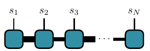
Each square here represents a rank-3 tensor (rank-2 for the left and right boundaires) \(A_{\alpha_j\alpha_{j+1}}^{s_j}\):
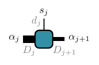
As before the vertical lines represent the physical indices. The new horizontal lines are called ancillary indices, with the physical and ancillary indices at each site \(j\) labelled by \(s_j,\alpha_j\) respectively. A connecting line between two tensors (squares) represents a contraction over the common index of the two tensors. A varying width of the ancillary legs represents the fact that each dimension can be different (their labels are in gray). With this convention, the MPS diagram above is a rigorous representation of the mathematical expression
where \(\{ \alpha \} = \{ \alpha_1, \ldots, \alpha_{N-1}\}\), and \(\alpha_i \in \{1 \cdots D_i \}\).
In this tutorial we will take all \(D_i\) (also called bond dimension) equal to a single \(D\) . Any tensor can be written as an MPS by means of the Singular Value Decomposition (although at the cost of very high bond dimensions –exponentially high as \(N\to \infty\))
We begin by creating directly the node structure of the MPS. First we define functions to build each block of the MPS and then the MPS itself:
# Retrieving a component

def block(*dimensions):
  '''Construct a new matrix for the MPS with random numbers from 0 to 1'''
  size = tuple([x for x in dimensions])
  return np.random.random_sample(size)

def create_MPS(rank, dimension, bond_dimension):
  '''Build the MPS tensor'''
  mps = [
      tn.Node( block(dim, bond_dim) )] +
      [tn.Node( block(bond_dim, dim, bond_dim)) for _ in range(rank-2)] +
      [tn.Node( block(bond_dim, dim) )
      ]

  #connect edges to build mps
  connected_edges=[]
  conn=mps[0][1]^mps[1][0]
  connected_edges.append(conn)
  for k in range(1,rank-1):
      conn=mps[k][2]^mps[k+1][0]
      connected_edges.append(conn)

  return mps, connected_edges
We will calculate the memory size of MPS of different dimensions and ranks (notice we are able to go much farther than before)
dimensions = range(2,9,2)
MPS_ranks = range(2,150)
MPS_memory = []

for dim in dimensions:
    bond_dim = 2
    MPS_memory = []
    for i in range(len(MPS_ranks)):
        rank = MPS_ranks[i]

        # Creating the MPS state:
        ##################################################################
        mps_nodes, mps_edges = create_MPS(rank, dim, bond_dim)
        MPS_memory.append(np.sum([x.tensor.nbytes for x in mps_nodes]))

    # Plot Results
    plt.loglog(MPS_ranks, MPS_memory, 'o',ls=':', label = f'd = {dim}')

plt.legend()
plt.xlabel('Tensor Rank')
plt.ylabel('MPS memory')

plt.show()
We obtain the following results:
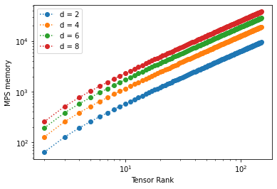
We see that memory requirements drop significantly: the scaling is now \(\sim N\) (which is polynomial). We can probe higher physical dimensions with less memory.
Retrieving components of a MPS
Let us now retrieve a component of a system of physical dimension \(2\) and rank \(N=20\). This is equivalent to accessing the components of the wavefunction of a 1D quantum chain of \(20\) qubits! The main computational cost will be the contraction of the MPS bonds. Here we use a simple algorithm to perform the calculation: contract each bond successively until the entire MPS has collapsed to the desired component of the tensor.
With this scheme one can calculate a component of the tensor in a time linear in \(N\).
########################################################################
#----- Retrieving a Component from an MPS by Contracting its edges-----#
########################################################################
dim = 2
bond_dim = 2
rank = 20
components=tuple(np.random.randint(0, dim, rank)) #select randomly the components that we will retrieve
print(f'components are: {components}')

mps_nodes, mps_edges = create_MPS(rank, dim, bond_dim)
for k in range(len(mps_edges)):
    A = tn.contract(mps_edges[k])

#the last node now has all the edges corresponding to the tensor components.

print(f'coefficient of the tensor at the selected components: {A.tensor[components]}')
Using the TensorNetwork library
TensorNetwork offers a simple built-in MPS class which can be used for tensor network calculations, which we will use in the following. Retrieving a component is again simply done by contracting over ancillary indices of the MPS. We’ll write the entire algorithm for \(\textsf{N} = 24\) and \(d = d_i = 2\) (again to make reference to spins):
#Component Retrieval Algorithm:

rank = 24
phys_dim = 2
bond_dim = 6

# build the mps:
# the state is canonically normalized when we define the class FiniteMPS
mpstate = tn.FiniteMPS.random(
  d = [phys_dim for _ in range(rank)],
  D = [bond_dim for _ in range(rank-1)],
  dtype = np.float32,
  canonicalize=True
  )

# connect the edges in the mps and contract over bond dimensions
nodes = [tn.Node(tensor,f'block_{i}') for i,tensor in enumerate(mpstate.tensors)]

connected_bonds = [nodes[k].edges[2] ^ nodes[k+1].edges[0] for k in range(-1,rank-1)]

for x in connected_bonds:
 contracted_node = tn.contract(x) # update for each contracted bond

# evaluate at a desired component
component = tuple(np.random.randint(0,phys_dim,rank))

print(f'Selected components of tensor: {component}')
print(f'Corresponding coefficient of tensor: {contracted_node.tensor[component]}')
MPS form a special class of 1-dimensional quantum wave functions which are only weakly entangled. In 1 spatial dimension, there is a rigorous proof that ground states of gapped local Hamiltonians can be approximated to arbitrary accuracy by an MPS with finite bond dimension \(D\). Conversely, for any MPS one can construct a local gapped Hamiltonian which has this MPS as its ground state (called a parent Hamiltonian).
Inner Product of MPS
Inner products appear all when calculating expectation values and norms of quantum states. They are sometimes called overlaps. Notice that the MPS structure makes the inner product of tensors graphically intuitive, involving the contraction of all the connected edges and bonds:
An efficient algorithm takes advantage of the factorization properties of the resulting matrices once the tensors have been put into an MPS form. We make the contractions in a “edge-bond-bond” sequence, sweeping along the graph:
np.random.seed(3) # fix seed to build the same tensors each time random is called

phys_dim = 2
bond_dim = 2
ranks = range(2, 60)

for phys_dim in range(2, 11, 2): # check how physical dim changes scaling
  overlap = []
  for rank in ranks:
      mpstateA = tn.FiniteMPS.random(d = [phys_dim for _ in range(rank)], D = [bond_dim for _ in range(rank-1)], dtype = np.complex128)
      mpstateB = tn.FiniteMPS.random(d = [phys_dim for _ in range(rank)], D = [bond_dim for _ in range(rank-1)], dtype = np.complex128)
      nodesA = [tn.Node(np.conj(tensor), f'A{i}') for i, tensor in enumerate(mpstateA.tensors)]
      nodesB = [tn.Node(tensor, f'B{i}') for i, tensor in enumerate(mpstateB.tensors)]
      nodesA[0][0] ^ nodesB[0][0]
      nodesA[-1][2] ^ nodesB[-1][2]
      [nodesA[k][2] ^ nodesA[k+1][0] for k in range(rank-1)]
      [nodesB[k][2] ^ nodesB[k+1][0] for k in range(rank-1)]
      [nodesA[k][1] ^ nodesB[k][1] for k in range(rank)]
      contraction = nodesA[0] @ nodesB[0]
      for i in range(1, len(nodesA)):
          contraction = contraction @ nodesA[i] @ nodesB[i]
      overlap.append(np.abs(contraction.tensor))

  plt.loglog(ranks,overlap,'o',ls=':')
plt.show()
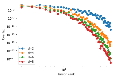
Notice how the overlap vanishes as the rank of the tensor grows. If we take the inner product of an MPS with itself we obtain the square of the norm, which is \(1\) for a normalized state.