Block sparse tensor networks
Some tensor networks are made of symmetric tensors: tensors that are left invariant when we act on their indices with transformations that form a symmetry group. For instance, a tensor can be invariant under the action of the \(Z_2\) group (corresponding e.g. to spin flip symmetry in a system of Ising spins), or of the \(U(1)\) group (corresponding e.g. to particle number conservation in a system of particles), or the \(SU(2)\) group (corresponding e.g. to spin isotropy in a system of quantum magnets). The symmetry group can be Abelian or non-Abelian. In an Abelian group, such as \(Z_2\) or \(U(1)\) all transformations commute, whereas in a non-Abelian group, such as \(SU(2)\), some transformations do not commute.
In a tensor that is symmetric under the action of a group, the symmetry can be exploited to obtain a more efficient, block-sparse representation, in which a fraction of the coefficients of the tensor are zero and do not need to be stored in memory. Moreover, the manipulation of symmetric tensors, including tensor-tensor multiplication and tensor decompositions (such as a QR or singular value decomposition) can be also implemented more efficiently by focusing directly on the non-vanishing coefficients of the tensor.
In this tutorial we explain our implementation of block sparse tensors within the TensorNetwork library. Currently, block sparsity support is restricted to Abelian groups.
If you are in a hurry, here are the most important points of our block-sparse tensor implementation:
- support for all abelian symmetries (implementation of new abelian symmetries is very easy)
- everything is numpy behind the scenes
- we use a so called element-wise encoding strategy to store non-zero tensor elements. This is different from other libraries like e.g. ITensor, where non-zero elements are stored in a block-by-block fashion in contiguos memory locations (block-wise encoding). For tensor networks with high-order tensors (e.g. PEPS or MERA) and many simultaneous symmetries, element-wise encoding typically is substantially more efficient than block-wise encoding.
- we have added a new
symmetricbackend to the library that should be used for symmetric tensor networks - we do currently not support jax, tensorflow or pytorch for block-sparse tensor networks
Symmetric tensors
An in-depth discussion of symmetries in quantum mechanics is way beyond the scope of this turorial. If you’re interested to dive deeper into this you’ll find some references at the end of the notebook. Instead, we’ll give here a minimal introduction to abelian symmetries in tensor networks, just enough to get you started. We will also only focus on Abelian symmetries (non-Abelian symmetries are more complicated and currently not supported). The following figure shows a symmetric tensor \(T_{ij}\) of order 2 (i.e. a matrix):
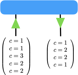
There is quite a bit of information in this picture, and we will cover it bit by bit. The matrix is represented by the blue rectangle, and its legs are represented by the two black lines. This is standard notation so far. For symmetric tensors, each leg needs two additional pieces of information.
- The indices of each leg have an integer charge \(c\) associated with it. These charges are shown in round brackets for each leg. So the index values of the first (left) leg \(i\) have charges \(c=\{1,1,3,2,2\}\) for the index values \(i = \{0,1,2,3,4\}\), while the index values of leg \(j\) have charges \(c=\{1,2,2,1\}\) for \(j=\{0,1,2,3\}\)
- Each tensor leg carries an \(\color{green}{\textbf{arrow}}\) (shown in green) indicating if the charges are “inflowing” or “outflowing”. In more formal lingo, we call a leg with an inflowing arrow a regular leg and one with an outflowing arrow a dual leg. Thus, leg \(i\) is regular while leg \(j\) is dual.
There are many different types of symmetries, giving rise to different
types of charges. For the sake of simplicity we will only consider so
called \(U(1)\) symmetries in the following. The corresponding
\(U(1)\) charges can take values \(c \in \mathbb{Z}\). In a
symmetric tensor, only those tensor elements are non-zero for which the
inflowing and outflowing charges are conserved. In the above example
these are the elements (0,0), (0,3), (1,0), (1,3), (3,1), (3,2), (4,1),
(4,2). All other elements are identically zero. Our BlockSparseTensor
class takes advantage of this by storing only the non-zero elements of
the tensor, together with the charges and arrows. The two main
advantages of this data model are that
- memory requirements are considerably reduced by storing only non-zero elements. For tensors with many simultaneous symmetries the memory reduction can be a factor of a 100 or more.
- certain operations, like tensor contractions and matrix factorizations, can be substantially sped up (up to a factor of 100) by letting them operate on the smaller symmetryblocks of non-zero elements of the tensor instead of the full tensor itself which would include all elements that are identically zero.
Our block-sparse tensor code is organized around the following three main classes:
BaseCharge
We use a BaseCharge type to store
charge information, i.e. the integer values of charges, their duality
transformation and their fusion properties. Actual charge types like
e.g. U1Charge are derived from the BaseCharge type.
Index
We use an Index type to bundle the charge and flow
information of a tensor leg. The Index type is a convenience class.
We use False and True to encode inflowing and outflowing arrows,
respectively.
BlockSparseTensor
This type represents a symmetric
tensor. It stores the charge and flow information (together referred to
as meta-data) of the tensor legs, and holds the non-zero elements of the
tensor in a 1d numpy array. Where possible, we have tried to keep the
API of BlockSparseTensor identical to numpy’s ndarray.
To initializate a random BlockSparseTensor (the preferred way of
initialization), we need to define the charge and flow information and
pass it to the constructor of BlockSparseTensor. Let’s initialize a
tensor with the above shown charges:
import tensornetwork as tn
from tensornetwork import BaseCharge, U1Charge, Index, BlockSparseTensor
import numpy as np
c_i = U1Charge([1,1,3,2,2]) #charges on leg i
c_j = U1Charge([1,2,2,1])   #charges on leg j
print(c_i)
print(c_j)
#use `Index` to bundle flow and charge information
i = Index(charges=c_i, flow=False) #We use `False` and `True` to represent inflowing and outflowing arrows.
j = Index(charges=c_j, flow=True)
tensor = BlockSparseTensor.random([i,j], dtype=np.complex128) #creates a complex valued tensor
<class 'tensornetwork.block_sparse.charge.U1Charge'>
charges:
array([[1, 1, 3, 2, 2]], dtype=int16)

<class 'tensornetwork.block_sparse.charge.U1Charge'>
charges:
array([[1, 2, 2, 1]], dtype=int16)
The non-zero elements are stored in the attribute
BlockSparseTensor.data. We can check that there are indeed only 8
non-zero elements
print(tensor.data)
[0.84753142+0.22766597j 0.65268088+0.8616853j  0.38187661+0.9934243j
 0.69947644+0.02371861j 0.4538116 +0.84746537j 0.64808382+0.11478288j
 0.65378104+0.44730301j 0.0092896 +0.44352757j]
We can also export tensor to a dense numpy.ndarray (including
the zero elements) using todense(), which reveals the
“block-structure” of the tensor. Be careful though when exporting large
tensors, because this can consume a lot of memory.
print(tensor.todense())
[[0.84753142+0.22766597j 0.        +0.j         0.        +0.j
  0.65268088+0.8616853j ]
 [0.38187661+0.9934243j  0.        +0.j         0.        +0.j
  0.69947644+0.02371861j]
 [0.        +0.j         0.        +0.j         0.        +0.j
  0.        +0.j        ]
 [0.        +0.j         0.4538116 +0.84746537j 0.64808382+0.11478288j
  0.        +0.j        ]
 [0.        +0.j         0.65378104+0.44730301j 0.0092896 +0.44352757j
  0.        +0.j        ]]
BlockSparseTensor can be reshaped just like numpy arrays.
i0 = Index(U1Charge.random(19,-3,3), flow=False)
i1 = Index(U1Charge.random(20,-3,3), flow=False)
i2 = Index(U1Charge.random(21,-3,3), flow=False)
a1 = BlockSparseTensor.random([i0,i1,i2], dtype=np.float64)
#reshaping behaves just as expected, with the exception that the
#elementary shape of the tensor has to be respected
a2 = a1.reshape((19*20, 21))
print('shape of a2:', a2.shape)
a3 = a2.reshape((19,20*21))
print('shape of a3:', a3.shape)
a4 = a3.reshape((19,20,21))
print('shape of a4:', a4.shape)
shape of a2: (380, 21)
shape of a3: (19, 420)
shape of a4: (19, 20, 21)
There are limitations to reshaping. In essence, you can only reshape a
BlockSparseTensor into a shape that is consistent with its
“elementary” shape, i.e. the shape at initialization time. This is a
notable difference to numpy arrays. For example, while reshaping of
a1 into a shape (19,2,10,21) would be possible if a1 was a
dense numpy.ndarray, it is no longer possible for
BlockSparseTensor because we don’t have the neccessary information
to split up i1 into two seperate legs. If you try anyway, we’ll
raise a ValueError:
a5 = a1.reshape((19,2,10,21))
---------------------------------------------------------------------------

ValueError                                Traceback (most recent call last)

--> 1 a5 = a1.reshape((19,2,10,21))
tensornetwork/block_sparse/blocksparsetensor.py in reshape(self, shape)
    257       raise ValueError("The shape {} is incompatible with the "
    258                        "elementary shape {} of the tensor.".format(
--> 259                            tuple(new_shape), tuple(flat_dims)))
    260
    261     if np.any(new_shape == 0) or np.any(flat_dims == 0):


ValueError: The shape (19, 2, 10, 21) is incompatible with the elementary shape (19, 20, 21) of the tensor.
Transposing tensors also works as expected:
b1 = a1.transpose((0,2,1))
print('shape of b1', b1.shape)
b2 = b1.transpose((1,2,0))
print('shape of b2', b2.shape)
shape of b1 (19, 21, 20)
shape of b2 (21, 20, 19)
transpose and reshape can be composed arbitrarily:
b3 = a1.reshape([19*20,21]).transpose([1,0]).reshape([21,19,20])
print('shape of b3:', b3.shape)
shape of b3: (21, 19, 20)
transpose and reshape both act only an a tensor’s meta-data and are thus essentially
free operations (i.e. no computational cost).
To contract two tensors, their flow and charge information has to match.
A leg with an outflowing arrow can only be contracted with a leg with an
inflowing arrow. In the following snippet, A.conj() is the complex
conjugate of tensor A. Complex conjugation of a
BlockSparseTensor flips the arrows (i.e. reverses the flows) on each
leg.
import time
D0,D1,D2,D3=100,101,102,103
i0 = Index(U1Charge.random(D0,-5,5), flow=False)
i1 = Index(U1Charge.random(D1,-5,5), flow=False)
i2 = Index(U1Charge.random(D2,-5,5), flow=False)
i3 = Index(U1Charge.random(D3,-5,5), flow=False)
A1 = BlockSparseTensor.random([i0,i1,i2,i3])
t1 = time.time()
A2=tn.block_sparse.tensordot(A1,A1.conj(),([0,1],[0,1])) #conj() returns a copy with flipped flows
print('sparse contraction time: ', time.time() - t1)
print('shape of A2:', A2.shape)
sparse contraction time:  0.3365299701690674
shape of A2: (102, 103, 102, 103)
We can compare the runtime of the sparse contraction with the dense one. On a 2018 macbook pro the sparse contraction is more than 20 times faster than dense contraction:
Adense = np.random.rand(D0,D1,D2,D3)
t1=time.time()
A2dense=np.tensordot(Adense,Adense,([0,1],[0,1]))
t2=time.time()
print('dense contraction time:  ', t2-t1)
dense contraction time: 7.412016868591309
Some matrix factorizations are also supported. We currently support
svd, eig, eigh and qr. If you need more submit an issue
on our github page and we’ll try to implement it! Here is an example of
an sv decomposition:
A2 = A2.reshape([D2*D3, D2*D3])
U,S,V = tn.block_sparse.svd(A2) #S is a 1d `ChargeArray` object, not a `BlockSparseTensor`.
check = A2 - U @tn.block_sparse.diag(S) @V #this should be all 0
print('||A2 - U @ diag(S) @ V||: ',np.linalg.norm(check.todense()))
A remark is in order here. While U and V above are regular
BlockSparseTensor objects, S is of a different type
ChargeArray that holds the singular values of A2 in a 1d
array-like object. ChargeArray is a base class of
BlockSparseTensor. The function tn.block_sparse.diag() takes
either a 1d ChargeArray and constructs a 2d BlockSparseTensor,
or it takes a 2d BlockSparseTensor and extracts its diagonal into a
1d ChargeArray. tensordot contractions (and almost all other
routines) should only be used on BlockSparseTensor (unless
explicitly stated otherwise).
Here are the other available matrix factorizations:
eta, U = tn.block_sparse.eig(A2) #eta is a 1d `ChargeArray` object, not a `BlockSparseTensor`.
check = A2 - U @tn.block_sparse.diag(eta) @ tn.block_sparse.inv(U)
print('||A2 - U @ diag(eta) @ inv(U)||: ',np.linalg.norm(check.todense()))#this should be close to 0

Q,R = tn.block_sparse.qr(A2) #QR decomposition
check = A2 - Q@R #this should be all 0
print('||A2 - Q @ R||: ',np.linalg.norm(check.todense()))

#eigh decomposition
tmp = BlockSparseTensor.random([i1,i1.copy().flip_flow()])
herm = tmp + tmp.conj().T #create a hermitian matrix

eta, U = tn.block_sparse.eigh(herm) #eta is a 1d `ChargeArray` object, not a `BlockSparseTensor`.
check =herm - U @tn.block_sparse.diag(eta) @ U.conj().T
print('||A2 - U @ diag(eta) @ herm(U)||: ',np.linalg.norm(check.todense()))#this should be close to 0
||A2 - U @ diag(eta) @ inv(U)||:  1.7393301276315685e-07
||A2 - Q @ R||:  2.7049451996920878e-09
||A2 - U @ diag(eta) @ herm(U)||:  0.0
As you probably noticed, BlockSparseTensor can be added and
subtracted, given that their meta-data is matching:
i0 = Index(U1Charge.random(10,-3,3), flow=False)
i1 = Index(U1Charge.random(11,-3,3), flow=False)
i2 = Index(U1Charge.random(12,-3,3), flow=False)
B1 = BlockSparseTensor.random([i0,i1,i2])
B2 = B1 + B1 #matching meta-data
A ValueError will be raised if the meta-data is not matching
B3 = B2 + B1.transpose((0,2,1)) #raises an error
---------------------------------------------------------------------------

ValueError                                Traceback (most recent call last)

--> 1 B3 = B2 + B1.transpose((0,2,1)) #raises an error


tensornetwork/block_sparse/blocksparsetensor.py in __add__(self, other)
    596
    597   def __add__(self, other: "BlockSparseTensor") -> "BlockSparseTensor":
--> 598     self._sub_add_protection(other)
    599     #bring self into the same storage layout as other
    600     _, index_other = np.unique(other.flat_order, return_index=True)


tensornetwork/block_sparse/blocksparsetensor.py in _sub_add_protection(self, other)
    570       raise ValueError(
    571           "cannot add or subtract tensors with shapes {} and {}".format(
--> 572               self.shape, other.shape))
    573     if len(self._charges) != len(other._charges):
    574       raise ValueError(


ValueError: cannot add or subtract tensors with shapes (10, 11, 12) and (10, 12, 11)
Doing things like B1 += 1 is currently not supported since this
would violate the charge conservation.
BlockSparseTensor.sparse_shape returns a list[Index] that can be
used to initialize a new BlockSparseTensor. Note that the flows of
the legs of the new tensor will be identical to the flows of the
original tensor on the respective legs.
D0,D1,D2,D3=100,101,102,103
i0 = Index(U1Charge.random(D0,-5,5), flow=False)
i1 = Index(U1Charge.random(D1,-5,5), flow=False)
i2 = Index(U1Charge.random(D2,-5,5), flow=False)
i3 = Index(U1Charge.random(D3,-5,5), flow=False)
A = BlockSparseTensor.random([i0,i1,i2,i3])
B = BlockSparseTensor.random([A.sparse_shape[0], A.sparse_shape[1]])
print('shape of B: ', B.shape)
shape of B: (100, 101)
Index objects can also be multiplied, which allows to do the following:
C = BlockSparseTensor.random([A.sparse_shape[1]*A.sparse_shape[2], A.sparse_shape[0]])
print('shape of C: ', C.shape)
shape of C: (10302, 100)
You can flip flows of an Index in place using Index.flip_flow().
To obtain a copy of the index with flipped flow, use
Index.copy().flip_flow():
sparse_shape = A.sparse_shape
print('flows of indices of A:', [i.flow for i in sparse_shape])
flipped = [i.copy().flip_flow() for i in sparse_shape]
print('flows of copied indices of A:', [i.flow for i in flipped])
flows of indices of A: [[False], [False], [False], [False]]
flows of copied indices of A: [[True], [True], [True], [True]]
The symmetric backend in TensorNetwork
We have added a symmetric backend to TensorNetworks which can be
used to construct symmetric tensor networks.
tn.set_default_backend('symmetric')

i0 = Index(U1Charge.random(1000,-3,3), flow=False)
i1 = Index(U1Charge.random(100,-3,3), flow=False)
i2 = Index(U1Charge.random(1001,-3,3), flow=False)
A1 = BlockSparseTensor.random([i0,i1,i2])

#tensordot-style contraction
A2=tn.block_sparse.tensordot(A1,A1.conj(),([0,1],[0,1]))

#ncon style contraction on tensors
A3 = tn.ncon([A1, A1.conj()],[[1,2,-1],[1,2,-2]])

#ncon style contraction on nodes
node = tn.Node(A1)
node2 = tn.ncon([node, tn.conj(node)],[[1,2,-1],[1,2,-2]])


print('shape of node2: ',node2.shape)
print('||A3 - A2||: ', np.linalg.norm((A3 - A2).todense())) #should be close to 0
print('||node2.tensor - A2||: ', np.linalg.norm((node2.tensor - A2).todense())) #should be close to 0
shape of node2:  (1001, 1001)
||A3 - A2||:  0.0
||node2.tensor - A2||:  0.0
The usual TensorNetwork API is also available:
n1 = tn.Node(A1)
n2 = tn.Node(A1.conj())
n1[0] ^ n2[0]
n1[1] ^ n2[1]
result = n1 @ n2
print(np.linalg.norm((node2.tensor - result.tensor).todense()))
0.0
For example, splitting nodes is carried out in the exact same way as for dense (non-symmetric) tensors.
#split node into two nodes
U1, U2,_ = tn.split_node(n1,[n1[0], n1[1]], [n1[2]])
print(np.linalg.norm((U1 @ U2).tensor.todense() - n1.tensor.todense()))
7.057099298396375e-12
#split node using svd
U1, S,U2,_ = tn.split_node_full_svd(n1,[n1[0], n1[1]], [n1[2]])
print(np.linalg.norm((U1 @S@ U2).tensor.todense() - n1.tensor.todense()))
7.048166180740012e-12
Implementing your own symmetry
In order to implement your own symmetry you need to define a new class
of charges. To illustrate the concept we’ll show how to implement a new
class Z3Charge (even though it’s already supported in the library).
You can find more example code in tensornetwork/block_sparse/charge.py.
Any custom charge type needs to implement the three static methods
fuse, dual_charges and identity_charge.
fuse(charge1, charge2: provides the implementation of charge fusiondual_charges(charge): provides the implementation of duality transformation of chargesidentity_charge: returns the identity charge for the charge type
We don’t have to implement Z3Charge.__init__, even though in general
it’s encouraged to do it in order to perform checks. If you provide it,
be sure to maintain the same function signature (including default
values) as in BaseCharge. super().__init__(...) should always be
called as shown below.
class Z3Charge(BaseCharge):
    """
    We represent Z3 charges as integer values from the set {-1,0,1}

    Charge fusion is:
    -1 + -1 ->  1
     1 +  1 -> -1
    -1 +  1 ->  0
     1 + -1 ->  0
     1 +  0 ->  1
    -1 +  0 -> -1
     0 + -1 -> -1
     0 +  1 ->  1
     0 +  0 ->  0

    Charge duality is:
    -1 ->  1
     0 ->  0
     1 -> -1

    Identity charge is 0
    """
    def __init__(self,
                 charges,
                 charge_labels = None,
                 charge_types = None,
                 charge_dtype=np.int16) -> None:
        """
        perform checks here
        """
        super().__init__(
            charges,
            charge_labels,
            charge_types=[type(self)],
            charge_dtype=charge_dtype)

    @staticmethod
    def fuse(charge1, charge2):
        return np.mod(np.ravel(np.add.outer(charge1 ,charge2))+1,3) - 1
    @staticmethod
    def dual_charges(charge):
        return -charge #for this representation, duality is negation of the sign
    @staticmethod
    def identity_charge():
        return np.int16(0) #the identity charge for our representation if `0`
    @classmethod
    def random(cls, dimension, minval=-1, maxval=1):
        """
        convenience function for initialization of random charge
        """
        if minval < -1 or minval > 1:
            raise ValueError("minval has to be between -1 and 1")
        if maxval < -1 or maxval > 1:
            raise ValueError("minval has to be between -1 and 1")

        charges = np.random.randint(minval, maxval + 1, dimension, dtype=np.int16)
        return cls(charges=charges)
That’s it, we’re ready to use the symmetry.
tn.set_default_backend('symmetric')
i0 = Index(Z3Charge.random(100,-1,1), True)
i1 = Index(Z3Charge.random(100,-1,1), False)
i2 = Index(Z3Charge.random(100,-1,1), True)

D = BlockSparseTensor.random([i0,i1,i2])
result = tn.ncon([D, D.conj()], [[1,2,-1],[1,2,-2]])
References
- Howard Georgi, Lie Algebras in Particle Physics, Frontiers in Physics
- https://arxiv.org/abs/1008.4774
- https://arxiv.org/abs/1208.3919
- https://arxiv.org/abs/1202.5664